MDfit
A computational method for constructing atomic models from cryo-EM and biochemical data
Description of the Approach
Molecular assemblies are intrinsically dynamic and often have many functionally-relevant configurations that are only transiently populated. Direct structural methods (such as x-ray crystallography and cryogenic-electron microscopy) can not typically capture the atomic details of these configurations, since they do not correspond to minima on the energy landscape. However, cryo-EM and x-ray methods can describe configurations that are partially consistent with these transient configurations. In addition, non-structural methods (such as chemical probing) may complement this data by providing signatures of particular structural features in these transient configurations.The MDfit methodology allows you to incorporate data from x-ray crystallography, cryo-EM and biochemical studies in order to prepare atomic models that are consistent with transient configurations. When using the MDfit method, one begins with a structure-based model (provided by the smog-server.org server or SMOG 2). By definition, the initial configuration (obtained from x-ray/cryo-EM, or other methods) is defined as the lowest energy configuration (red line in figure). If a simulation is performed with the structure-based forcefield alone (at low enough temperatures), it will provide you with a description of the fluctuations about the initial basin.
If cryo-EM data is available for an alternate configuration (or a sub-region of your complex), you can add another energetic term that will bias the structure towards the cryo-EM density (green line in figure). If the cryo-EM term of the forcefield is included with a large energetic weight, then the total potential energy surface will be "downhill" (blue line) with the target (cryo-EM) configuration at the bottom of the new energetic minimum. Since the target is a minimum on the energy landscape, performing simulations with this new forcefield will result in the system moving into the target configuration. When you have additional information about your target system (perhaps for regions that lack an EM density), then restraints may be introduced via a variety of types of interactions (i.e. harmonic, 6-12, etc). Again, when simulations are performed with the combined structure-based/EM-restraint forcefield, the system can relax into configurations that are consistent with all of these contributions.
Downloading the code
The MDfit method has been implemented in a modified version of Gromacs (Version 4.5.5), which can be downloaded here. CAUTION: Unless you have used MDfit in Gromacs Version 4.5.5, please read all instructions on this page. In addition, this code is provided as a courtesy. It is not under development, nor is it actively supported as part of the SMOG suite of software.Quick Tutorial
Notes on compiling and using this code:
- You must compile and run with MPI support. Typically, assemblies studied by EM methods are large enough that the SMOG models will scale perfectly when the interconnect between cores is fast (i.e. cores on the same board, or Infiniband connected). We have found that when dynamic load balancing is employed, many systems scale to roughly 200-300 atoms/core.
- Notes on compiling can be found here.
- The simulated map is calculated on a single processor, which can lead to the map calculations being rate limiting. For this reason, it is often advantageous to only calculate the simulated map every N steps. We have found that N=100-1000 gives consistent end-state models for multiple systems, but the value most appropriate for your system will depend on the strength of the energetic term associated with the map.
- This code has been tested on MAC OSX 10.8.2 (64 bit Intel) and several Linux distributions.
To get you started, we will take you through an example that uses MDfit ported to Gromacs V4.5.5, in conjunction with smog-server V1.2.X.After installing the code on your local machine, follow these steps to perform a modeling simulation with MDfit. Here, we will walk you through an example fit for Adenylate Kinase. Adenylate Kinase is a 3-domain protein that undergoes a large structural rearrangement upon ligand binding. In this example, we will start with the "open" conformation of AKE (PDB: 4AKE), and we will fit it to a theoretical density generated from the "closed" conformation (PDB: 1AKE).
- Download a PDB file (or, use any other PDB-formatted structure) For this example, PDB entry 4AKE is used. In this PDB file there are 2 copies of AKE. Since the EM density only includes 1 molecule, remove 1 copy from the file (for example 4AKE.single.pdb).
- Prepare your EM density For this exercise, use this density (1AKE.density.sit). If your density map is not in Situs format (.sit), you will need to reformat it. Commonly, one has a .brix file. To convert to Situs format, we load the brix file into Chimera. In Chimera, go to "Volume->Volume Viewer". Inside of the Volume Viewer window, go to "File->Save map as...". Select your new file name and select File Type "MRC". Using the map2map module of Situs, convert the MRC file to a Situs file. There may be simpler ways to convert brix files to Situs files, but this will get the job done. For convenience, we highly recommend that at this point you reset the origin of the map to 0,0,0 (this is part of the first line in the .sit file).
- Perform an initial rigid-body alignment of the atomic model to the target density This may be performed manually (as done here), or you can use automated alignment methods. For this exercise, we provide a manually-aligned structure (4AKE.aligned.pdb).
- Generate the topology and coordinate files for your system, using the SMOG webtool. When using the SMOG tool, it is important to select the checkbox for option 6 (i.e. do not recenter the system). Since you have already aligned the system to your map, this option will prevent any unwanted translations in the coordinates. Here are output topology (4AKE.top) and coordinate (4AKE.gro) files generated by the SMOG server, using default energetic values and contact map.
- Organize the mdp file For the tutorial, use the provided mdp file (MDfit-gmxV4.5.5.sample.mdp). Take a careful look at these mdp settings, as they determine how MDfit is applied.
- Prepare your tpr file Now, you have all the necessary files to perform your first fit. The grompp module (the MDfit-modified version) will be used to generate a .tpr file. Here is a sample grompp command:
grompp -f MDfit-gmxV4.5.5.sample.mdp -c 4AKE.gro -p 4AKE.top -o 4AKE.MDfit.tpr
- Perform the fit With the MDfit-modified Gromacs, perform the simulation:
mpirun -np 4 mdrun -v -s 4AKE.MDfit.tpr -emf 1AKE.density.sit -noddcheck -dd 2 2 1
On most modern machines, this calculation should only take a few minutes. On a MacBook Air, with a single dual-core 2 GHz Intel i7 processor, this calculation required 45 seconds.
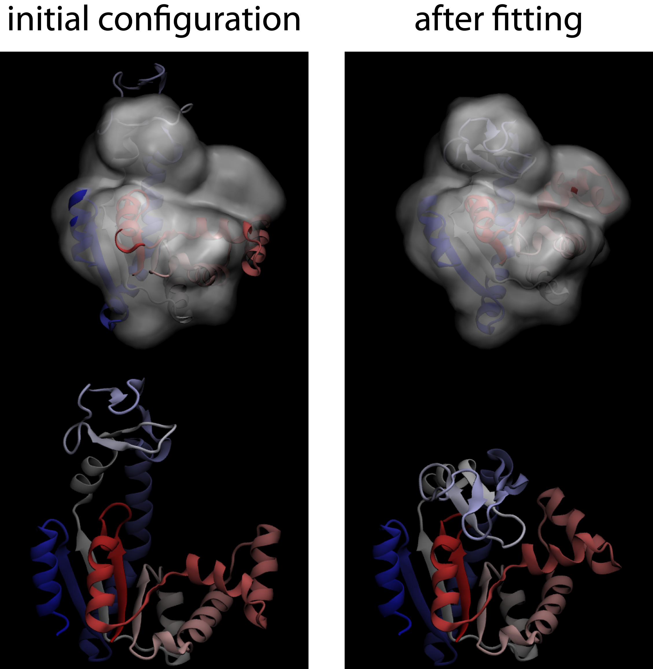
- Check the results You can view the fitting simulation using VMD. You can check the quality of the fit, for this example, by comparing it to the closed conformation of AKE (1AKE). If you perform an rmsd alignment of the C-alpha atoms, the final configurations of the fit should be ~ 1.5 Å from the closed configuration. Your results should look like the following figure.
Download Structural Models
In Whitford et al, PNAS 2011, it is indicated that the structural models are freely available. Since the associated webpage no longer exists, we have made them available here.
This resource is provided by the Center for Theoretical Biological Physics.
Please direct questions and comments to info@smog-server.org.
Page created and maintained by Jeff Noel and Paul Whitford